This collaboration with the University of Southampton used Raman spectroscopy to investigate cores from an ancient climate event. The study was published in Geochemical Perspectives Letters.
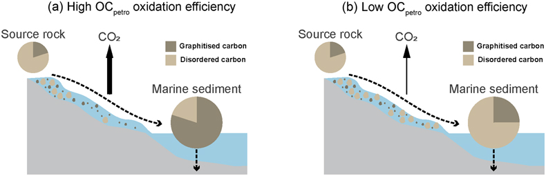
The PETM event caused major, rapid global warming of 4-6 °C, which also released large amounts of carbon into the atmosphere. The climate change associated with the event altered hydrological cycles and may have driven erosion and degradation of petrogenic organic carbon (OCpetro), which may have been a further positive feedback in the PETM climate system.
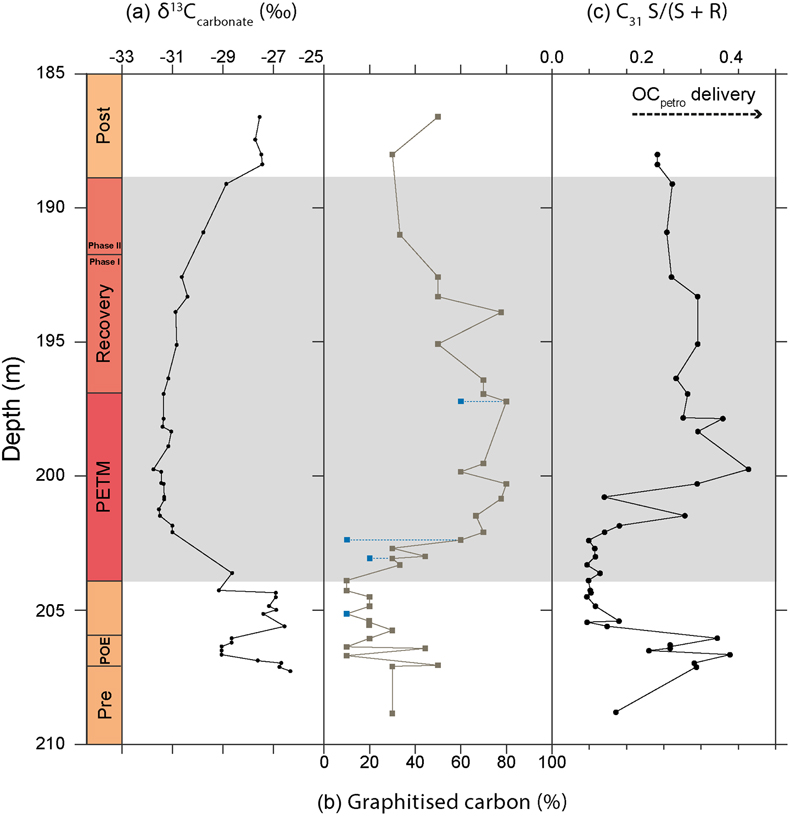
This is the first study to use Raman spectroscopy to investigate OCpetro oxidation at the PETM. We found that there was an increased contribution of graphite during the PETM, likely caused by intensified physical erosion and enhanced OCpetro oxidation.
In areas where there is a range of OCpetro inputs, both graphitic and disordered, Raman spectroscopy appears to be a very promising tool for investigating past changes in the carbon cycle.
This paper shows how organic carbon, when deeply buried and transformed into graphite, can survive multiple cycles of erosion, transport and burial. It is available, open-access, from the journal website.
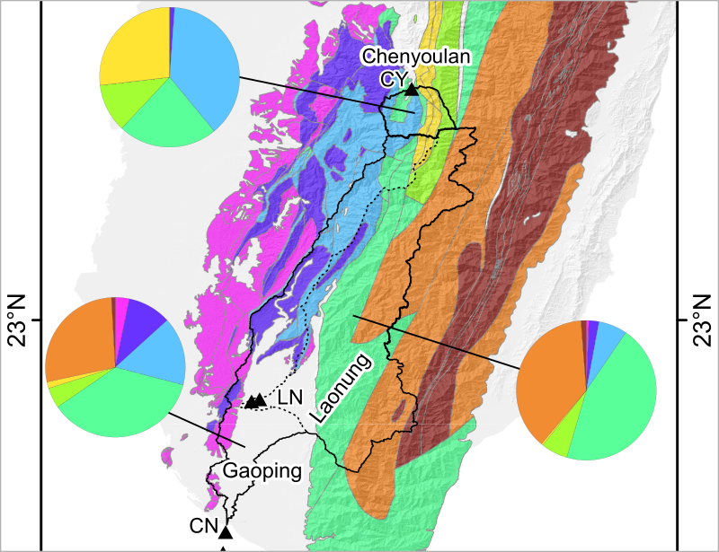
River catchments in southwestern Taiwan contain lots of different rock formations
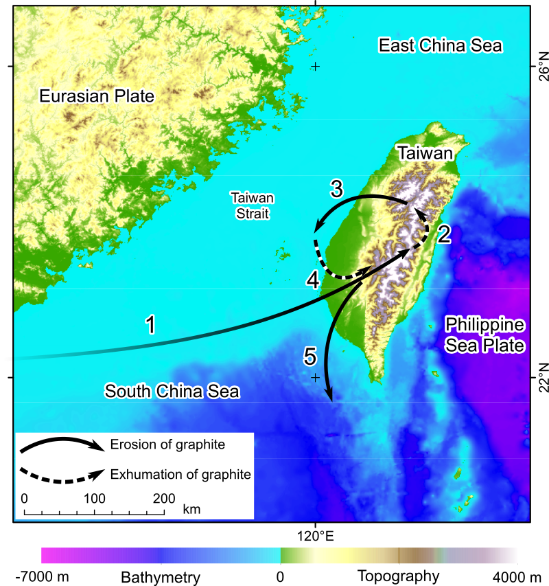
The samples came from Taiwan, which has a pretty extreme tectonic and climatic setting. The convergence of the Eurasian and Philippine Sea plates leads to rapid mountain building, and the impact of severe typhoons each year leads to large amounts of erosion. This means that lots of sediment is removed from the island each year, including from rocks that were previously buried deep under the island, and metamorphosed. I looked at samples collected from several river catchments in the southwestern part of the island, and from some offshore cores. Some of these catchments drained the Central Range mountains, and others the Western Foothills and Coastal Plain. The rocks in these two regions are very different, especially in terms of the carbon they contain.
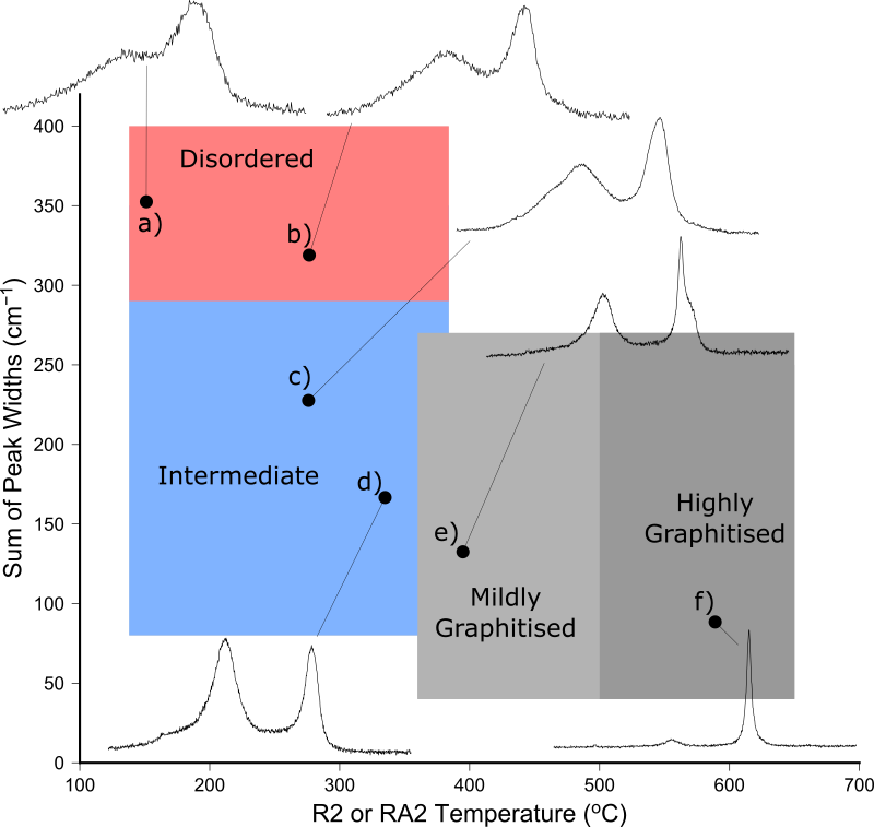
Differentiating betwen graphitic and disordered carbon using Raman spectra
The analytical work was based around the Raman spectroscopy technique I developed during my PhD (published back in 2013). Raman spectra were collected from particles of organic carbon in the sediments, and automatically processed to determine which Raman peaks were present, where they were located, how tall and how wide they were. The peaks found in each sample were used to show the types of carbon present in each rock. As each particle is analysed independently, there is no averaging effect if a samples is a mixture of several sources.
This analysis showed that rivers draining the youngest rocks, which had experienced the least metamorphism, had the most graphite in. The rivers draining the most metamorphic rocks had little or no graphite. This could only be explained if the graphite was eroded from somewhere else and then deposited into the Taiwanese sediments before they became rocks. The graphite-rich rocks were sourced from Taiwan itself – the rapid tectonic uplift means that a lot of material has been removed from the top of the mountains and washed into the surrounding ocean. Yet there are no rocks in Tawain that have been buried deep enough to make graphite, so the original graphite must have come from somewhere else entirely!
Three phases of graphite erosion (arrows 1, 3 and 5) and two of exhumation in the island of Taiwan (arrows 2 and 4)
Our best guess is that China was the original graphite source, since there are lots of graphite bearing outcrops in the regions near to Taiwan, eroding into the South China Sea. So the first phase of recycling was from China out onto the ocean floor before Taiwan became an island. Once the island appeared out of the ocean, the second phase of erosion moved these graphite rich sediments from the newly formed land back into the nearby seas (the second recycling phase). These rocks were then uplifted themselves, forming the Western Foothills of the island, and are now eroding for the third time out into the South China Sea. During all this time, some of the graphite has survived, and can be seen easily in the modern sediment.
All this means that graphite crystals are pretty stable, and can survive being eroded, transported and buried in sediments multiple times. They can be used as tracers, because although the rock they came from has been broken up into tiny pieces and dispersed across the ocean floor, each graphite flake can be characterised very precisely by Raman.
Turning organic carbon into graphite also gives it stability, stopping it from degrading back into carbon dioxide. On long timescales, this means that carbon is transferred from the atmosphere into the biosphere (trees and plants), and then into the lithosphere (rocks) where it can survive for millions of years.
Update: The paper is now published and can be downloaded from the journal webpage.
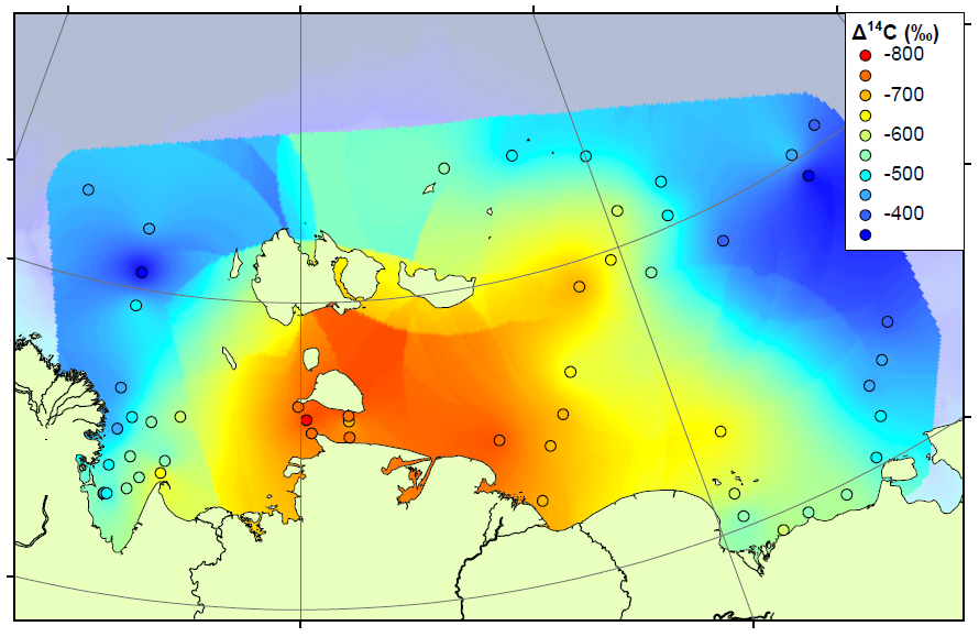
Map of radiocarbon ages across the ESAS
The study continues our work on the East Siberian Arctic Shelf, and contains two new datasets. The first is a radiocarbon study, measuring the age of organic matter on the shelf using carbon dating (see map above). By measuring the age, we can determine whether the carbon has come from the ocean (very young), the topsoil (quite young) or the coastal permafrost (thousands of years old). We combined our results with those already measured on the shelf to form the most complete radiocarbon map for this area. The high-resolution map shows that areas close to the shore and away from the major rivers are home to very old carbon, almost certainly sourced by erosion of old permafrost cliffs. Elsewhere on the shelf, the carbon is younger but not as young as modern topsoils or ocean carbon. Therefore the coastal erosion carbon is having an influence right across the shelf.
A pyrolysis probe can heat samples to 900 C in milliseconds
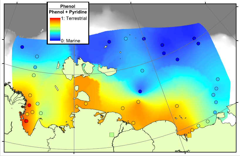
Our second technique is pyrolysis GCMS, where samples are smashed into small pieces using high temperatures and the small pieces are then analysed using GCMS. This technique generates a large amount of small pieces, too many to analyse each one individually, and so we decided to concentrate our efforts on a few target molecules. These included Phenols, which are probably sourced from lignin, a major component of land plants, and Pyridines, which are nitrogen-containing compounds probably sourced from proteins. We think that a lot of the Pyridines in the Arctic Ocean will come from organisms living in the ocean itself, and therefore the Pyridines are a potential tracer for marine organic matter. By comparing the concentrations of Phenols and Pyridines, we can estimate the amount of terrestrial and marine organic carbon in a sample.
Phenol-Pyridine ratio on the Arctic Shelf
In the map above, red areas are dominated by Phenols and are therefore rich in terrestrial carbon, blue areas are dominated by Pyridines and are therefore rich in marine carbon. This pattern matches very well with our previous work in the region, showing that there is a transition from terrestrial to marine conditions across the Arctic Shelf, and that the transition zone lasts for hundreds of kilometres offshore. This means that there is a lot of terrestrial carbon being deposited, and hopefully buried, on the shelf, rather than all of the eroded carbon being degraded and released as CO2.
This paper was published in Organic Geochemistry, and is available open-access through the journal website and the MMU e-space repository. In the paper we take a detailed look at lipid biomarkers along a transect from the Kolyma River to the Arctic Ocean.
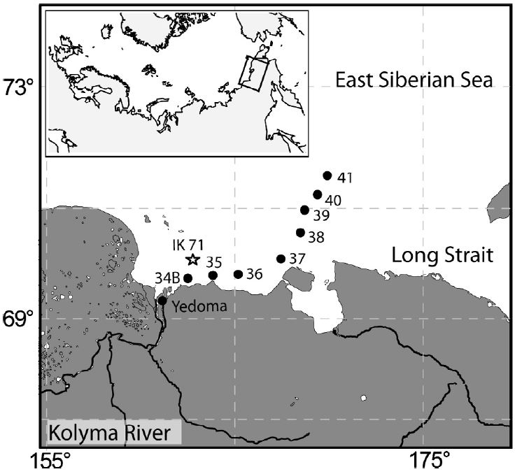
The data used in this paper is a subset of the data from across the East Siberian Artic Shelf (ESAS) published shortly afterwards in Biogeosciences. In this paper we took a closer look at the offshore trends seen in material delivered to the ocean by the Kolyma River, the easternmost of the Great Russian Arctic Rivers. The Kolyma River catchment is entirely underlain by continuous permafrost, which makes this are an extreme endmember in terms of permafrost systems. The main sources of organic matter from the Kolyma region are river erosion, mostly from top few metres of soil, the active layer that freezes and thaws each year, and coastal erosion from the “yedoma” cliffs along the shoreline.
Sample locations for the Kolyma River – ESAS transect
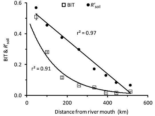
These samples had previously been analysed for bulk properties (total organic carbon content, carbon isotope ratios) and some basic biomarker measurements, but we added complex lipid analyses to the story. We measured both GDGT and BHP lipids, these are found in microbes and can be analysed using LCMS. Amongst the many applications of these lipids, they can be used to trace the amount of soil found in offshore sediments. Each group of molecules has an index associated with it: GDGTs are used in the BIT index and BHPs are used in the R’soil index. Values of 0 would have no soil input and 100% marine carbon, while values towards 1 would be dominated by soil.
Offshore trends in the BIT and R’soil indices
Usually these indices show the same offshore trends, which would be expected since they are both supposed to be tracing the same number – the proportion of carbon coming from soil. However, as the figure above illustrates, the two indicies have very different patterns from the river mouth (0 km) across the shelf (500 km). The BIT index drops quickly offshore, making a curved offshore profile, but the R’soil index forms a straight line offshore. Therefore two different techniques, supposedly measuring the same thing, don’t show the same results.
We think that this is due to the source of lipids used to make each index. Branched GDGTs (from soils) are common in sediments close to the river mouth, but their concentration drops quickly offshore. Marine GDGT concentrations increase across the shelf and this combination causes the BIT index to decrease rapidly. Branched GDGT concentrations in soils and lakes on land are high, but they are very rare in the coastal permafrost cliffs. Therefore any coastal erosion is not really affecting the BIT index.
On the other hand, soil marker BHP molecules are found in river sediment and coastal permafrost, and so there are two terrestrial sources. The concentration of soil marker BHPs drops much slower offshore than for the GDGTs. Also different, the concentration of the marine BHP marker doesn’t increase offshore. This combination means that the R’soil index drops much slower than the BIT index.
In the end, what this paper mainly shows is that when using biomarkers as proxy measurements for something else one single result is probably not enough. Proxy measurements are valuable tools, but they depend on measuring one thing to discover another. Combining multiple proxies together adds value and reliability to a study, either by confirming a hypothesis or bringing new insights.
This paper, led by Josh West and colleagues in Taiwan, was published in Limnology and Oceanography. The full text is available via the journal website, since all L&O papers become open access after three years.
The island of Taiwan, in the South China Sea, has an interesting, yet devastating, combination of climate, biology and geology. It sits on the plate boundary between Eurasia and the Phillipines, which are moving into each other and causing the island to rise out of the ocean. This leads to earthquakes as the land is pushed up, and rapid erosion as the mountains get steeper and taller. The mountain sides collapse as landslides, producing sediment that is prone to being washed away by Taiwan’s many rivers. These rivers may not be the longest in the world, but they carry a lot of water, because Taiwan sits in the tropical zone where the year-round high levels of rainfall are topped up by several typhoons each year. The final piece of this jigsaw is the biology – being in a warm, wet region means that Taiwan is very biologically productive, with extremely fast forest growth rates.
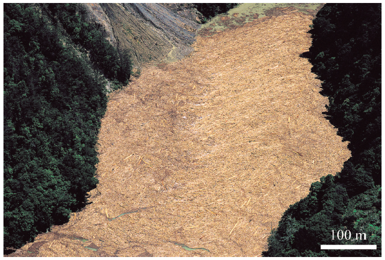
A Taiwanese reservoir after Typhoon Morakot
Coupling all of these features together leads to a heavily forested mountainous island on which the hillsides are regularly landsliding and generating woody debris (tree trunks, branches, shrubs etc.) The large typhoons that hit the island each year provide water which washes the woody debris into the rivers and then out to the ocean.
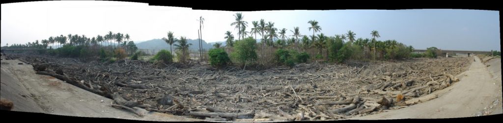
In 2009, Taiwan was struck by a particularly devastating tropical cyclone, Typhoon Morakot. The island received about 4 metres of rainfall in just a couple of days, enough to cause rivers to burst their banks, washing away entire villages and unfortunately leading to several deaths. I visited the island a few months later, and the clear-up operation was still going on. Beside the rivers was up to a metre of chaotic sediment with tree branches sticking out of it, since the waters had carried everything off the hillside and dumped it when the floods receded. A lot of the tree trunks made it all the way through the river, out to the sea. They washed up on the shoreline around Taiwan, and were reported as far away as Japan.
A Taiwanese river channel filled with logs after the storm
These trees contain a lot of carbon, which has been moved from the hillside to the floodplain and out to the sea. Our study tried to work out just how much carbon, in the form of coarse woody debris, was being transported during this storm. Single river channels, such as the picture above, could contain 40 million tonnes of carbon – how much carbon was washed away by the whole storm?
There were two independent methods used to make the carbon estimates. The first one compared aerial photography before and after the storm to look at how much area was affected by landslides, and how much of the island was covered in forest. If you combine the forest cover data with the landslide map, and correct for areas where landslides do not deliver the woody debris to the river network, an estimate of carbon mobilisation can be made
The second method used reservoirs as sampling facilities. Reservoirs have filters to stop large trees going through their exit pipelines, and so any woody debris reaching the reservoir will be stopped at the dam (see the top picture for an extreme example). Knowing the area of land that drains into the reservoir, and the amount of wood trapped at the dam, you can scale up to the area of the entire river catchment.
Both of these methods produced similar results, they agreed that there was a shocking amount of carbon washed to the ocean during the storm. The storm delivered 3.8 – 8.4 Teragrams of woody debris from Taiwan to the ocean, which represents 1.8 – 4.0 Teragrams of carbon. This is about 1/4 the annual delivery of carbon from the Amazon River, but most of that is as small particles. The woody debris delivery in these few days was over 10 times greater than the annual woody debris delivery from the Amazon. So one single event on a small island was significant from a global point of view, but how much carbon is a Teragram?
One Teragram is equal to one million tonnes; an oil tanker can carry 300 000 tonnes of oil (mostly carbon) and therefore the storm delivered 10 oil tankers worth of carbon to the ocean. Obviously this event is not as disastrous as an oil tanker spill – the woody material will rot down and provide food for ocean-living creatures as well as potentially being buried safely in the sediments.
Our paper shows just how much carbon can be washed away by a single storm, and highlights that large pieces of woody debris, too large to analyse by most techniques, are an important and probably under-studied element of the organic carbon cycle.
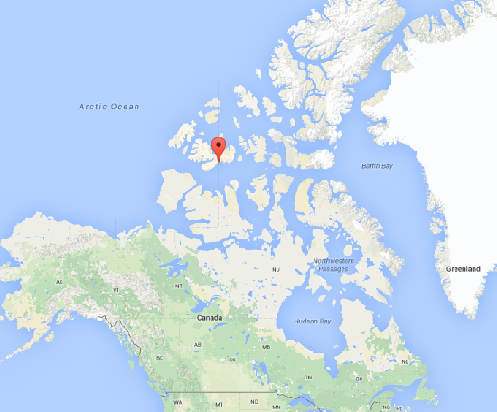
The February issue of “Organic Geochemistry” will include a paper by David Grewer and colleagues from the University of Toronto and Queen’s University, Canada which investigates what happens to organic carbon in the Canadian High Arctic when the surface permafrost layer slips and erodes. This is a paper that I was involved in, not as a researcher but as a reviewer, helping to make sure that published scientific research is novel, clear and correct.
Map of Cape Bounty in the Canadian High Arctic
The researchers visited a study site in Cape Bounty, Nunavut, to study a process known as Permafrost Active Layer Detachments (ALDs). The permafrost active layer is the top part of the soil, the metre or so that thaws and re-freezes each year. ALDs are erosion events where the thawed top layer is transported down the hillslope and towards the river. Rivers can then erode and transport the activated material downstream towards the sea.
The team used organic geochemistry and nuclear magnetic resonance spectroscopy to find out which chemicals were present in the river above and below the ALDs. The found that the sediment eroded from the ALDs contains carbon that is easily degraded and can break down in the river, releasing CO2 to the atmosphere and providing food for bacteria and other micro-organisms in the water.