permafrost – Defrosting the Freezer

Carbonaceous material export from Siberian permafrost tracked across the Arctic Shelf using Raman spectroscopy

In this paper, published in The Cryosphere, we used Raman spectroscopy to trace carbonaceous material from the shoreline to the furthest reaches of the East Siberian Arctic Shelf.

Raman spectroscopy uses laser light to determine the molecular structure of a wide range of materials. During my PhD, I showed that Raman could be used to probe individual particles of organic carbon to show whether they were disordered, like coal, or crystalline sheets of graphite. This collection of carbon particles, known as carbonaceous materials, are particularly hardwearing and resistant to breaking down during erosion and transport. During my post-doctoral research, I then used a range of organic geochemistry techniques to investigate the transition from terrestrial to marine carbon across the East Siberian Arctic Shelf, showing that coastal erosion and river erosion were both supplying organic matter to the ocean.

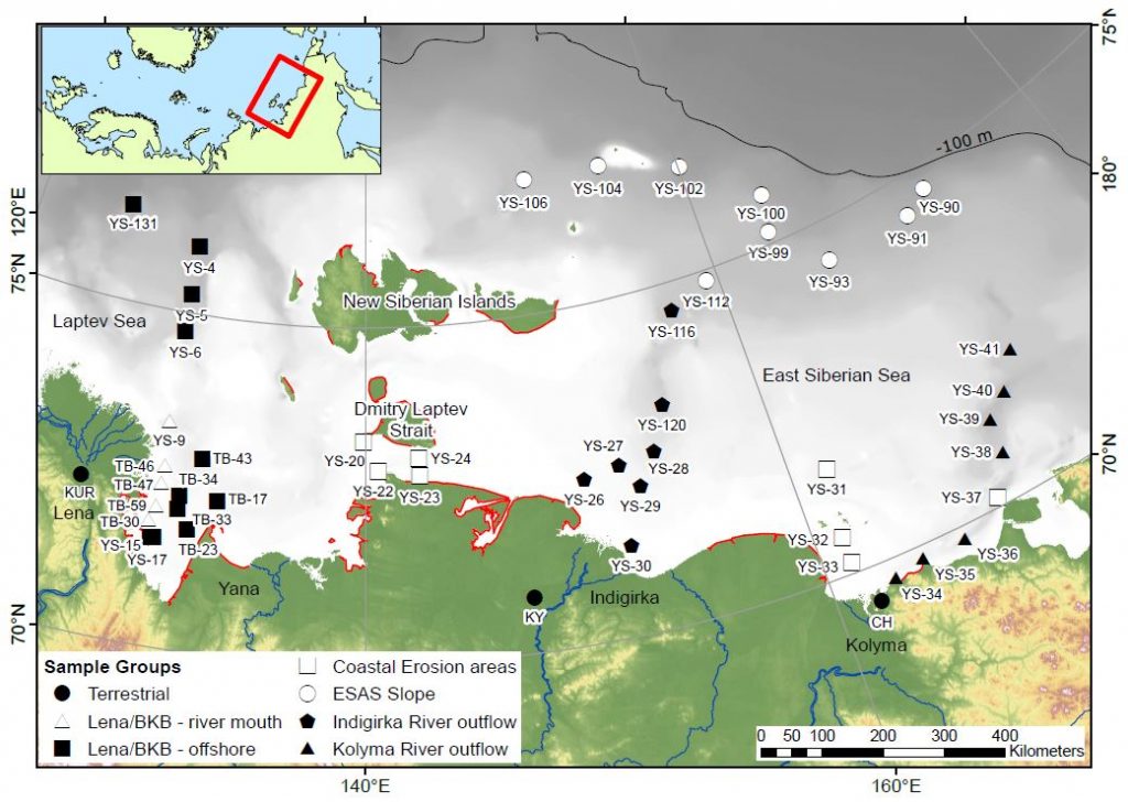
Map of the samples used in this study. Red lines are areas of intense coastal erosion

This study uses the Raman technique on those same Arctic Shelf sediments to look at the sources and distribution of carbonaceous material on the shelf. The samples used in our paper were collected from close to the mouths of some major rivers, from areas experiencing rapid coastal erosion, and from hundreds of kilometres offshore.

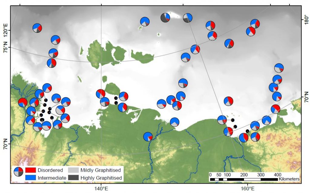
Groups of spectra found in the shelf samples

The hardest work, collecting over 1400 Raman spectra, was carried out by two undergraduate students, Melissa Maher and Jerome Blewett, who are co-authors on the paper. The collected spectra were then analysed using an automated peak fitting script, and grouped according to the shape of the fitted peaks. This provides an unbiased method for determining whether a carbon particle is highly graphitised, mildly graphitised, disordered, or somewhere in between. For each of the sites on the shelf we collected spectra from up to 30 particles, and looked at how many fitted into each group. Statistics were then used to spot patterns across the shelf.

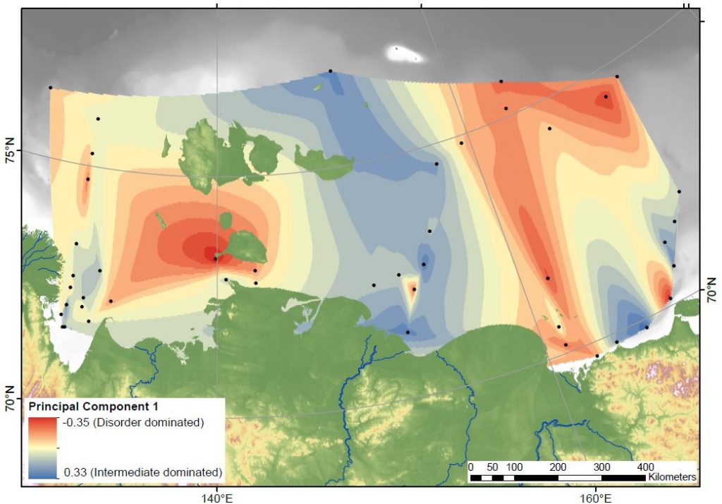
Distribution of "Disordered" and "Intermediate" carbon — Distribution of “Disordered” and “Intermediate” carbon

Our first finding is that the relative proportion of “disordered” and “intermediate” carbon particles varies, and that there are patches with more of one or the other group. At the coastline these patches align with two of the major rivers (Kolyma and Indigirka) and areas of rapid coastal erosion. Surprisingly, the patches can then be traced all the way across the shelf. We would have expected the currents in the ocean to have mixed the particles together further offshore, and in the biomarker studies we’ve done before we did not spot this kind of pattern. This means that Raman is a great way to trace the different sediment and carbon sources on the shelf.

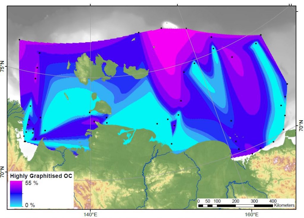
"Highly Graphitised" carbon is found in high proportions far offshore — “Highly Graphitised” carbon is found in high proportions far offshore

Our second finding is that the amount of “highly graphitised” carbon particles is highest in the furthest offshore samples. These very crystalline flakes of graphite are behaving differently to all the other carbon particle groups. It’s not clear exactly why this is, but one option is that everything else is breaking down and degrading before getting that far offshore. Or, the graphite particles could be so light that they sink very slowly, floating out to the shelf edge much easier than the other types.

This problem has implications for the global carbon cycle. These carbon particles have been released from permafrost on land and transported for hundreds of kilometres offshore, a trip that has taken thousands of years. If all of the carbonaceous material can survive the journey, it means that this fraction of the organic matter is not at risk of being degraded and released to the atmosphere as greenhouse gases. Burying it in the ocean provides protection from degradation for thousands or millions of years. Future studies should look at just how well the carbon particles can survive erosion and burial.

In summary, carbonaceous material is resilient to degradation and can be used to trace sediment sources across the Arctic shelf.

The Cryosphere, 12, 3293-3309, 2018
https://doi.org/10.5194/tc-12-3293-2018

Source, transport and fate of soil organic matter inferred from microbial biomarker lipids

06/09/2016 UPDATE: The paper has been accepted and is now published. The final version is available from the journal.

Our international team of East Siberian researchers currently has a paper in open review at Biogeosciences. The discussion paper, and its interactive comments, can be downloaded from the journal website.

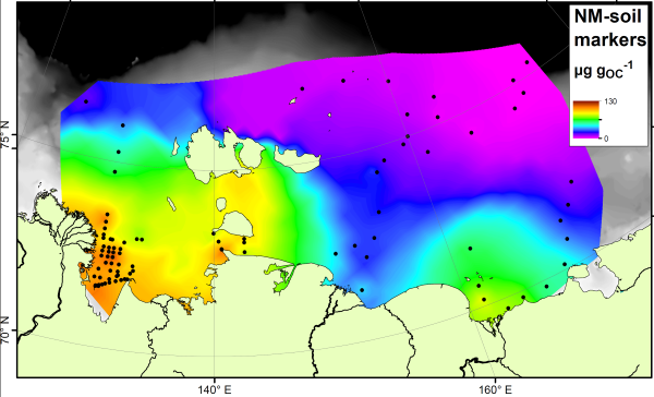
The paper studies a group of compounds called “bacteriohopanepolyols” (BHPs for short), which are found in the cell membranes of a range of microbes and are therefore one of the most common organic compounds around. They are found in modern and ancient sediments from all over the world. This study has concentrated on two groups of these. Group 1 is the soil marker compounds. These are only found in soils, and so have been used as tracers for soil material in rivers, lakes and offshore. Here is how they are spread across the East Siberian Artic Shelf:

BHPfig2a (Custom) — Soil marker compounds across the Arctic Shelf

Note how the soil marker concentrations are highest (orange colours) near to the rivers and coastlines. By measuring the concentration next to the river mouths, and in the sediments being washed away by coastal erosion, we show that it is not just rivers that are delivering the soil markers to the Arctic Ocean.

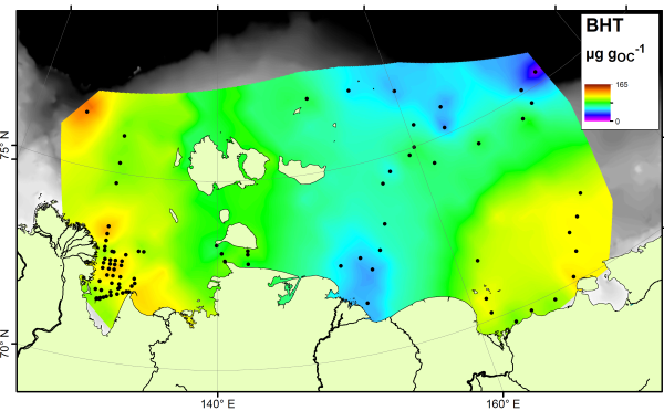
There is no single compound that is a true tracer for carbon produced in the ocean itself, but the compound bacteriohopanetetrol (BHT) is most abundant in marine settings despite being found in soils as well. Therefore if your sample is rich in BHT, and poor in soil markers, it is likely dominated by carbon from the ocean. Here’s a map of BHT across the East Siberian Arctic Shelf:

BHPfig2b (Custom) — BHT, a marine marker, is present across the Arctic Shelf

The BHT results show a fairly constant amount across the ocean floor. If we compare the soil marker concentrations to the BHT concentrations, we can see which areas are rich in soil carbon (more soil markers than BHT) and which are rich in marine carbon (more BHT than soil markers). This comparison is called the R’soil index, and is shown below:

R'soil index on the Arctic Shelf — R’soil index on the Arctic Shelf

The R’soil index shows that all along the East Siberian Arctic coastline, offshore sediments are dominated by carbon from the land. As you go further offshore, especially in eastern parts nearer to the Pacific Ocean, marine carbon is more important. This result shows a similar pattern to that seen using stable carbon isotopes, but is different to the pattern shown by the BIT index. Therefore these two indices, both based on microbial biomarkers, are tracing different parts of the carbon cycle.

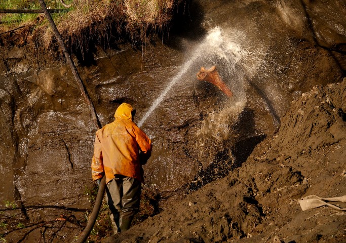
Ivory mining from thawing permafrost

The Guardian newspaper today reported on an interesting set of photographs today documenting one side effect of warming permafrost. Photographer Amos Chapple travelled to the East Siberian region to mine prehistoric ivory from permafrost. Locals had discovered tusks emerging from the river bank as rising temperatures coupled with erosion to uncover bones and tusks that had been buried for thousands of years.

A tusker excavates a prehistoric bone. Photo by Amos Chapple / RFE/RL

The photographs are well worth a look, documenting the extreme (and extremely dangerous) lengths that the ivory miners (“tuskers”) will go in order to find ivory worth tens of thousands of dollars per piece. They carve caverns into the permafrost using high pressure hoses, leaving behind a pock-marked hillside and a river full of debris.

A successful find will net more than $50 000 in cash, and the carved products will be sold for millions, likely in China. While the payback for the few who strike lucky can be life changing, the damage to the local ecosystem, and the likely increase in permafrost degradation and carbon release due to this activity, means that the long-term regional and global consequences will far outweigh the local gain.

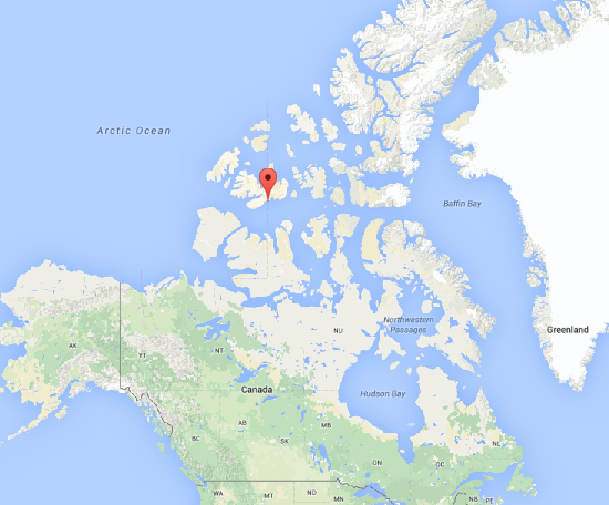
Canadian permafrost as a source of easily-degraded organic carbon

The February issue of “Organic Geochemistry” will include a paper by David Grewer and colleagues from the University of Toronto and Queen’s University, Canada which investigates what happens to organic carbon in the Canadian High Arctic when the surface permafrost layer slips and erodes. This is a paper that I was involved in, not as a researcher but as a reviewer, helping to make sure that published scientific research is novel, clear and correct.

Map of Cape Bounty in the Canadian High Arctic

The researchers visited a study site in Cape Bounty, Nunavut, to study a process known as Permafrost Active Layer Detachments (ALDs). The permafrost active layer is the top part of the soil, the metre or so that thaws and re-freezes each year. ALDs are erosion events where the thawed top layer is transported down the hillslope and towards the river. Rivers can then erode and transport the activated material downstream towards the sea.

The team used organic geochemistry and nuclear magnetic resonance spectroscopy to find out which chemicals were present in the river above and below the ALDs. The found that the sediment eroded from the ALDs contains carbon that is easily degraded and can break down in the river, releasing CO₂ to the atmosphere and providing food for bacteria and other micro-organisms in the water.

What Is: GRAR?

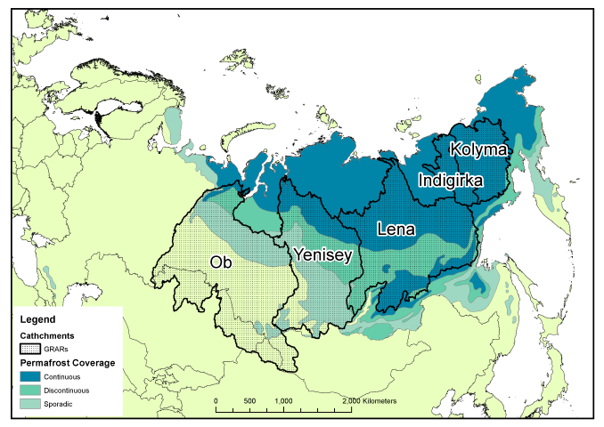
Russia is big, really big, and to go with that, it has some very big rivers. The majority of the Russian river outflow is into the Arctic Ocean, especially in the central and eastern parts of the country, and this is generally concentrated into a series of very large rivers. The largest of these are known as the Great Russian Arctic Rivers (GRARs). From west to east, these are the Ob, Yenisety, Lena, Indigirka and Kolyma, of which the Ob and Lena are largest, and Indigirka the smallest (small enough to not count in some people’s list of GRARs).

Catchment areas of the Great Russian Arctic Rivers

The Ob river is the world’s fifth-longest and has the sixth-largest drainage basin, yet has only the 19th highest annual discharge, being overtaken by the smaller Yenisey and Lena rivers to the east of it. All of these river basins contain some permafrosted land, which can reduce discharge during the winter months and have a very large flood-period in late spring / early summer when the meltwater arrives (the “freshet”).

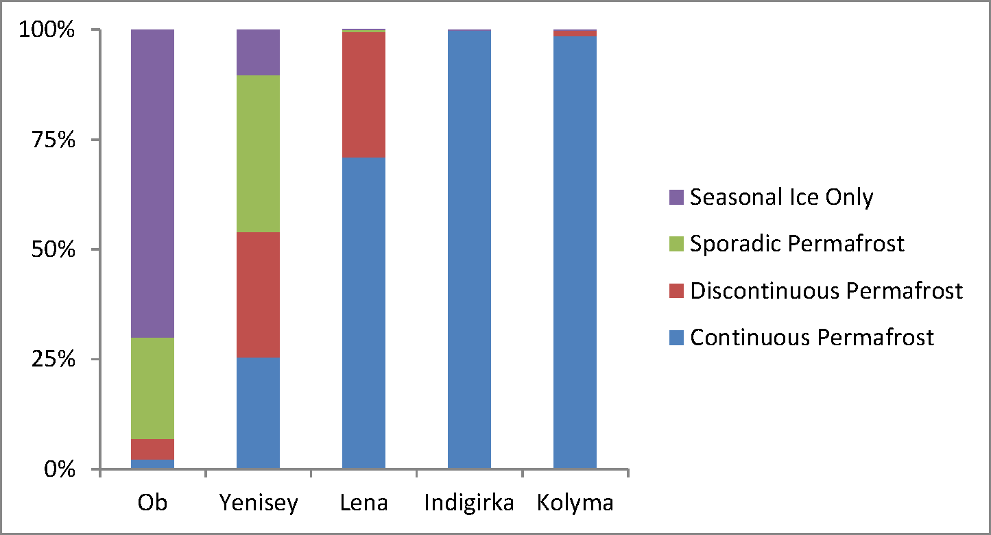
Permafrost within catchments of the GRARs

As the amount and continuity of permafrost increases from west to east, so the proportion of each permafrost type increases within the river basin. The Ob and Yenisey are largely free of continuous permafrost, allowing water to flow through the ground to the bedrock and into the river, whilst the Indigirka and Kolyma are practically 100% continuous permafrost, and thus any water discharging will have run along the top of the ground before entering the river itself. This can have consequences for the type of material, especially carbon, carried by the rivers.

Proportion of each type of permafrost within river basins

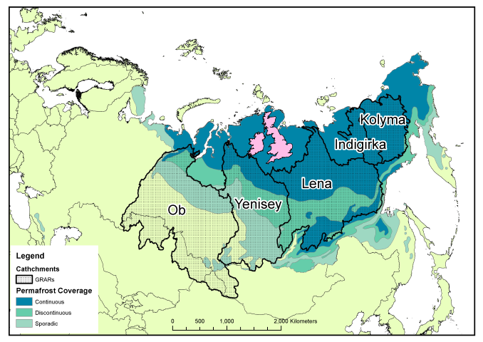
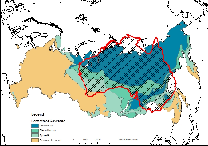
This east-west contrast is worth exploring in more detail in a later post, since it shows how Siberia may behave very differently if the permafrost were to thaw. As a final reminder of just how large the rivers are, even the smallest, Indigirka, manages to cover more area than the British Isles! As usual the full-resolution PDFs of the figures from this article can be downloaded here: River catchments no permafrost, Catchments and permafrost, Permafrost chart, Catchments and UK.

Comparing the catchment areas to the British Isles

Just how much permafrost is there?

The extent and type of Russian permafrost

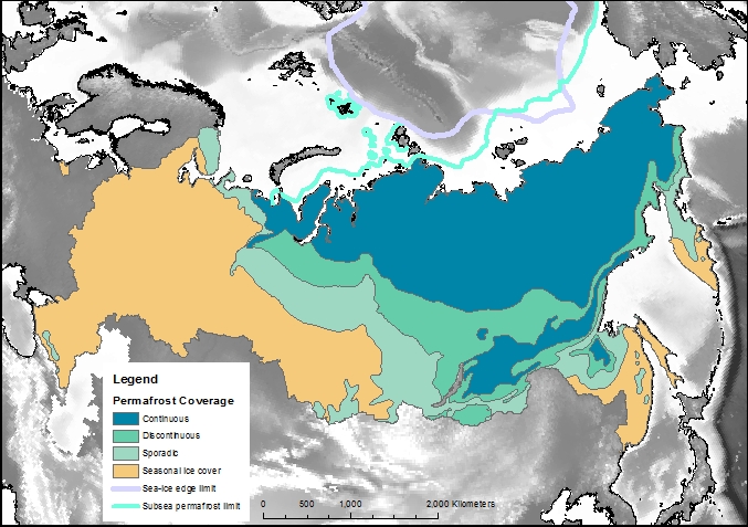
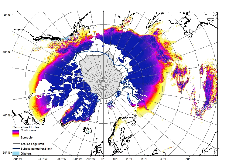
Permafrost covers 24% of the Earth’s northern hemisphere land surface, but how much is that? Well 24% corresponds to 23,000,000 km². That is a pretty big number, and doesn’t even count the subsea permafrost that covers lots of the Arctic Shelf (see the map above) so here are a few comparisons and measurements in less standard units.

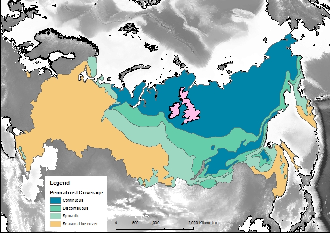
Great Britain compared to the Russian permafrost area.

Firstly, let’s compare the permafrost area to some other countries and continents. Here is Britain in comparison, at 243,000 km² it is almost inconsequential. Only one tenth of the northern hemisphere permafrost. Going up the scale Australia, with an area of 7,700,000 km², is one third of the northern hemisphere permafrost, and roughly the same size as the 7,400,000 km² that continuous and discontinuous permafrost represent in Siberia alone.

The land area of Australia compared to the Siberian permafrost

The maps above use data from the National Snow and Ice Data Centre

PDF versions are also available. Map1, Map2, Map3.

What is: Permafrost?

Permafrost is soil or sediment that is permanently below zero °C

When most people talk about permafrost, they think of frozen, empty soil with very little living on it, in it or near it. They think of a harsh, icy environment with glaciers, blizzards and possibly a few reindeer roaming around. But permafrost is much more varied than this. It does not necessarily have a covering of ice, but can be a thin layer of grass or peat with frozen soil underneath it, there can even be forests growing on the surface with frozen soil underneath them. There can be animals living on it, and bacteria living within the sediment. In fact, the permafrost might not even be on land! Here are just a little information about permafrost and what it contains.

Northern Hemisphere Permafrost. Also shown are subsea permafrost and the Arctic ice cap.

Permafrost soils, which are frozen so solid so you need a pneumatic drill to sample them, cover a quarter of the northern hemisphere land area, and can be up to 1500 m thick. They store more carbon than there is in the entire atmosphere. The very top layer will thaw each summer and freeze each winter, which allows plants to grow and animals to graze, but the lower parts remain frozen all the time. In the southern parts, there can be trees growing on top of the permafrost, this is known as the ‘taiga’. When it is too cold, and the growing season is too short, only grass, moss, shrubs and lichen can survive, this is the ‘tundra’.

Another example of permafrost is frozen methane-ice trapped on the seabed. Subsea permafrost is often ignored, but these icy crystals of frozen, flammable gas and water contain a large amount of trapped carbon, are prone to melting and gas release, and have been blamed for one of the most extreme climate events in geological history.

The last type of permafrost to be discussed here is ‘yedoma’. This is a feature of the very furthest reaches of the Arctic, and is formed by windblown dust freezing together to form a layer of dirty ice and sediment. These thick ice layers are often found on the Arctic coast, where they have no defences against the incoming waves from the Arctic Ocean and are eroded easily. As the Arctic warms, the sea ice that usually protects the coastline from the force of the waves is reduced to nothing, allowing the full power of the sea to erode into the shoreline

The map shown above can be downloaded here. The data was sourced from the University of Zurich Global Permafrost Zonation Index Map.