The February issue of “Organic Geochemistry” will include a paper by David Grewer and colleagues from the University of Toronto and Queen’s University, Canada which investigates what happens to organic carbon in the Canadian High Arctic when the surface permafrost layer slips and erodes. This is a paper that I was involved in, not as a researcher but as a reviewer, helping to make sure that published scientific research is novel, clear and correct.
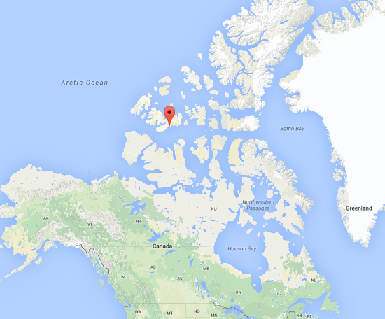
Map of Cape Bounty in the Canadian High Arctic
The researchers visited a study site in Cape Bounty, Nunavut, to study a process known as Permafrost Active Layer Detachments (ALDs). The permafrost active layer is the top part of the soil, the metre or so that thaws and re-freezes each year. ALDs are erosion events where the thawed top layer is transported down the hillslope and towards the river. Rivers can then erode and transport the activated material downstream towards the sea.
The team used organic geochemistry and nuclear magnetic resonance spectroscopy to find out which chemicals were present in the river above and below the ALDs. The found that the sediment eroded from the ALDs contains carbon that is easily degraded and can break down in the river, releasing CO2 to the atmosphere and providing food for bacteria and other micro-organisms in the water.
I will discuss Raman Spectroscopy in depth in a future post on this site, but the short version is that Raman allows me to determine the crystal structure of pieces of carbon within my samples. A river or marine sediment sample can be sourced from multiple areas, and mixed together during transport. Trying to work out where a sample was sourced from can prove very difficult. However, these source areas often contain carbon of different crystalline states; if I can identify the carbon particles within a sample then the sources of that sample, even if they have been mixed together, can be worked out. The challenge in this procedure is that there can be lots of carbon particles within a sample, and each one might be subtly different. To properly identify each mixed sample, lots of data is required, which can laborious to process.
Determining the types of carbon in a sample. Each spectrum is classified according to its peak shapes. Image (C) Applied Spectroscopy
My paper describes how lots of spectra can be collected efficiently from a powdered sediment sample. By flattening the powder between glass slides and scanning the sample methodically under the microscope, around ten high-quality spectra can be collected in an hour, meaning five to ten samples can be analysed in a day. Powdered samples are much easier to study than raw, unground, sediment, and I have shown that the grinding process does not interfere with the structure of the carbon particles, therefore it is a valid processing technique.
Once the data has been collected, I have devised a method for automatically processing the collected spectrum using a computer, which removes the time-consuming task of identifying and measuring each peak by hand. The peaks that carbon particles produce when analysed by Raman Spectroscopy have been calibrated by other workers to the maximum temperature that the rock experienced, and this allows me to classify each carbon particle into different groupings. These can then be used to compare various samples, characterise the source material and then spot it in the mixed samples.
Delegating as much analysis as possible to a computer ensures that each sample is treated the same, with no bias on the part of the operator, and also cuts down the time required to process each sample, which means that more material can be studied. The computer script used to analyse the samples is freely available and therefore other researchers can apply this to their data, enabling a direct comparison with any samples that I have worked on. This technique will hopefully prove useful to more than just my work in the future, and anyone interested in using it is welcome to contact me. While the paper discusses my application of the technique to Taiwanese sediments, I have already been using it to study Arctic Ocean material as well.
The paper itself is available from the journal via a subscription, and is also deposited along with the computer script in the University of Manchester’s open access library.
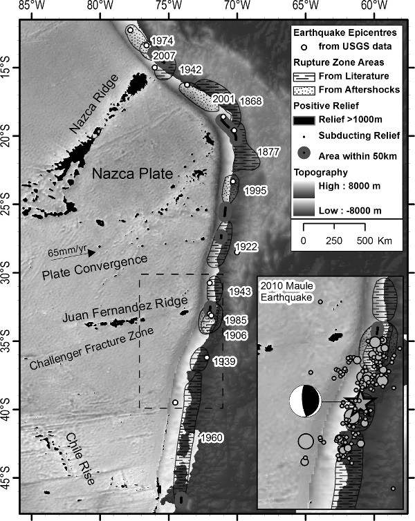
The initial observation for this work was that ‘great’ earthquakes, those which measured more than magnitude 8.0, tend to have end points in the same place. An earthquake end point is the limit to the earthquake fault plane movement, shaking will take place outside of this zone but it is most violent in the regions above the fault plate movement. The figure below shows the rupture zones and end points for great South American earthquakes.
Rupture zones and subducting topography in South America
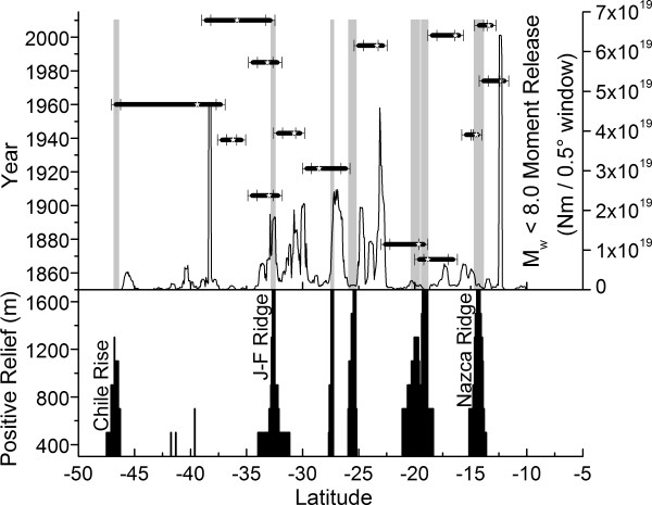
An initial inspection of the plate margin (where the incoming Pacific Plate is subducted underneath the South American Plate) suggested that when there are underwater mountains on the Pacific Plate coming into the subduction zone (black blobs on the figure above), these tend to match up with the end points of earthquakes. The figure below shows how topographic features (underwater mountains and ridges) match up with earthquake locations.
Subducting topography and earthquake locations
To test whether this was a real relationship, or just coincidence, I designed a model that produced earthquakes along the subduction zone. The model had two versions. In version one, earthquakes were placed in line along the subduction zone (as tends to happen in these situations, one earthquake starts at the end point of a previous one) but their end points were not constrained by anything. In the second version, if the earthquake tried to rupture past an incoming topographic feature, the rupture was stopped there.
By applying statistical tests to the model, I showed that the endpoints of earthquakes were far more likely than random chance to be located where topography > 1000m was being subducted. The model also showed that subducting topography led to a reduction in background earthquakes. At earthquake endpoints not associated with topography, there was an increased amount of smaller earthquakes releasing the built-up stress, but this was not seen at earthquake endpoints near to subducting topography. Therefore, subduction of a high seamount or ridge makes the subduction zone earthquake activity decrease (it becomes ‘aseismic’) which prevents both great earthquakes getting past, and smaller earthquakes from occurring.