Sometimes science involves £1 million machinery, exciting state-of-the-art laboratories, expensive and/or explosive chemicals, travel to far-flung exotic lands and schmoozing over canapes. Sometimes it involves retrieving some bits and bobs from a series of dusty drawers and bodging them together into something approximating workable equipment. Today was one of those days. I’ll explain Pyrolysis in a later post, but the aim of today’s work was to create an offline-pyrolysis set-up that can be used to prepare large quantities of sample for analysis later on. The pyrolysis oven itself was already in place, but a regular flow of nitrogen gas is needed to blow through it and transport the chemicals that are released.
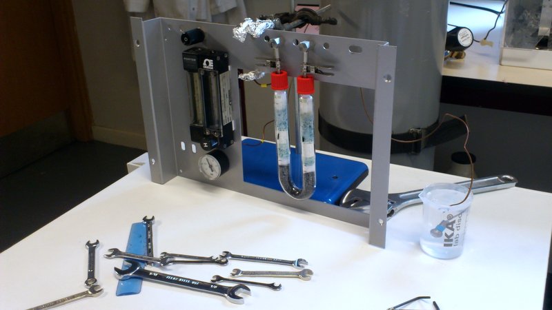
Delving around in the back of the lab, we managed to find the inner workings of an old carbon analysis machine sitting in pieces in a drawer. There were flow regulators; lots of copper pipes; a series of connecting nuts and bolts, of which most were incompatible with each other, but some that would play nicely; a couple of glass tubes filled with unknown solids; a pressure sensor; and a piece of steel that once lived inside the machine.
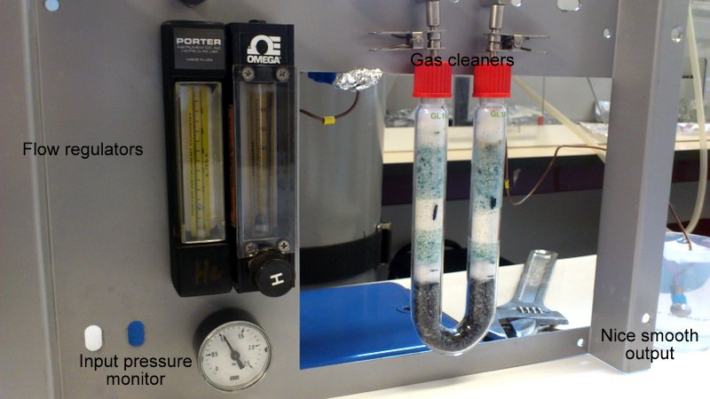
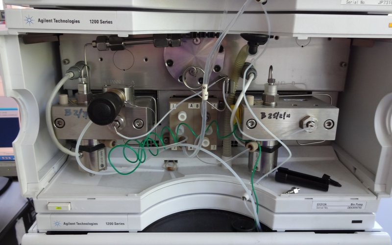
And here we have it! Gas comes from the bottle in the background into the first flow regulator. In an attempt at clarity and sensibility, this is the one on the right hand side, with the “H” dial on, since that’s the only way that the pipework at the back would work properly. At this point the input pressure from the bottle is measured as well, which will hopefully correspond nicely to the pressure measured from the regulator. This first regulator is more of a glorified tap, able to determine roughly how much gas comes through the system but not to accurately control the output rate.
Once the gas has flowed through here, the second flow regulator (on the left) has a much more precise knob (just out of shot above the word “PORTER”) that determines how much gas can flow through the rest of the system. This regulator also has a little floating ball gauge to show the flow rate.
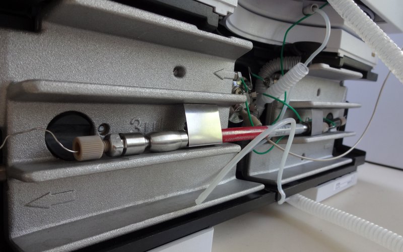
After that, the gas is cleaned in the u-bend. This will remove any liquid from the gas, so that it is nice and dry when it passes onto the samples, hopefully preventing them from reacting with the gas at all.
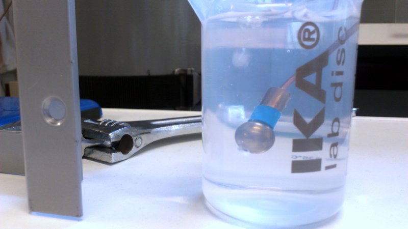
The last item on this test rig, is the output testing device. A glass of water.