This paper was published in the open access journal Earth Surface Dynamics, and is available through the journal website and the MMU e-space repository.
The paper is a combined effort from a large team of researchers interested in the way that organic carbon is exported from small tropical islands. These islands are very biologically productive, the forest grows quickly in the warm, wet climate. They are also responsible for delivering large amounts of sediment to the ocean. Rocks are weakened by earthquakes and then eroded by the frequent tropical storms that hit the islands. This washes sediment and carbon out to sea via two mechanisms. High sediment concentrations lead to ‘hyperpycnal’ plumes of material flowing along the ocean floor, lower sediment concentrations cause ‘hypopycnal’ flows that stay at the ocean surface. Both systems can spread sediments and carbon a long way offshore.
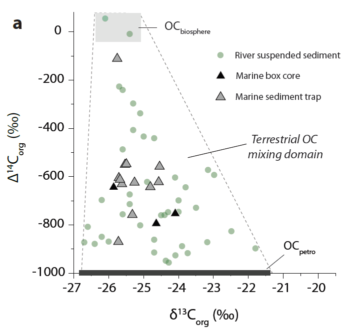
Marine sediment cores look very similar to the sediment coming out of the rivers
It had long been thought that hyperpycnal delivery of sediment, which usually only occurs in the most extreme weather conditions when floods deliver vast amounts of sediment to the ocean in a short period of time, were efficient methods of organic carbon preservation. Our data confirmed this hypothesis, showing that little terrestrial organic carbon was lost during transport, and little marine carbon added to the mixture.
However, the dataset also investigated how efficient hypopycnal delivery can be. Sediment and carbon are delivered throughout the year, in smaller floods and less extreme storms, and it had been suspected that this mechanism exposed the carbon to oxidising conditions where it could be degraded and released as CO2. We showed that in Taiwan, where hypopycnal conditions exist but are still receiving and accumulating a large amount of sediment, the burial efficiency of carbon in hypopycnal conditions is still very high. Marine carbon is mixed into the sediments, but at least 70% of the terrestrial carbon survives.
This means that small tropical islands are even better at exporting and burying carbon than was previously thought, and therefore better at sequestering atmospheric CO2. We estimated that more than 8 Teragrams (million tonnes) of carbon could be buried each year throughout Oceania.
This paper was published in Organic Geochemistry, and is available open-access through the journal website and the MMU e-space repository. In the paper we take a detailed look at lipid biomarkers along a transect from the Kolyma River to the Arctic Ocean.
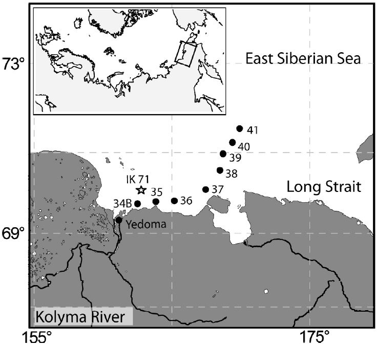
The data used in this paper is a subset of the data from across the East Siberian Artic Shelf (ESAS) published shortly afterwards in Biogeosciences. In this paper we took a closer look at the offshore trends seen in material delivered to the ocean by the Kolyma River, the easternmost of the Great Russian Arctic Rivers. The Kolyma River catchment is entirely underlain by continuous permafrost, which makes this are an extreme endmember in terms of permafrost systems. The main sources of organic matter from the Kolyma region are river erosion, mostly from top few metres of soil, the active layer that freezes and thaws each year, and coastal erosion from the “yedoma” cliffs along the shoreline.
Sample locations for the Kolyma River – ESAS transect
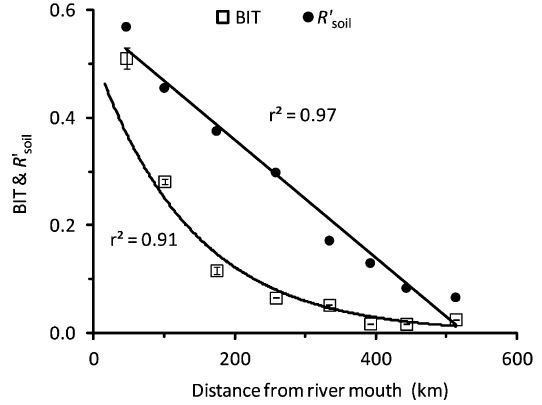
These samples had previously been analysed for bulk properties (total organic carbon content, carbon isotope ratios) and some basic biomarker measurements, but we added complex lipid analyses to the story. We measured both GDGT and BHP lipids, these are found in microbes and can be analysed using LCMS. Amongst the many applications of these lipids, they can be used to trace the amount of soil found in offshore sediments. Each group of molecules has an index associated with it: GDGTs are used in the BIT index and BHPs are used in the R’soil index. Values of 0 would have no soil input and 100% marine carbon, while values towards 1 would be dominated by soil.
Offshore trends in the BIT and R’soil indices
Usually these indices show the same offshore trends, which would be expected since they are both supposed to be tracing the same number – the proportion of carbon coming from soil. However, as the figure above illustrates, the two indicies have very different patterns from the river mouth (0 km) across the shelf (500 km). The BIT index drops quickly offshore, making a curved offshore profile, but the R’soil index forms a straight line offshore. Therefore two different techniques, supposedly measuring the same thing, don’t show the same results.
We think that this is due to the source of lipids used to make each index. Branched GDGTs (from soils) are common in sediments close to the river mouth, but their concentration drops quickly offshore. Marine GDGT concentrations increase across the shelf and this combination causes the BIT index to decrease rapidly. Branched GDGT concentrations in soils and lakes on land are high, but they are very rare in the coastal permafrost cliffs. Therefore any coastal erosion is not really affecting the BIT index.
On the other hand, soil marker BHP molecules are found in river sediment and coastal permafrost, and so there are two terrestrial sources. The concentration of soil marker BHPs drops much slower offshore than for the GDGTs. Also different, the concentration of the marine BHP marker doesn’t increase offshore. This combination means that the R’soil index drops much slower than the BIT index.
In the end, what this paper mainly shows is that when using biomarkers as proxy measurements for something else one single result is probably not enough. Proxy measurements are valuable tools, but they depend on measuring one thing to discover another. Combining multiple proxies together adds value and reliability to a study, either by confirming a hypothesis or bringing new insights.
This paper, with Jens Turowski and Bob Hilton, was recently published as an open-access article in Geology and is available from the journal website and via the MMU e-space repository. In it we show that erosion and transport of large woody material (coarse particulate organic carbon; CPOC) is very important in terms of the overall carbon cycle, but is concentrated in very extreme events.
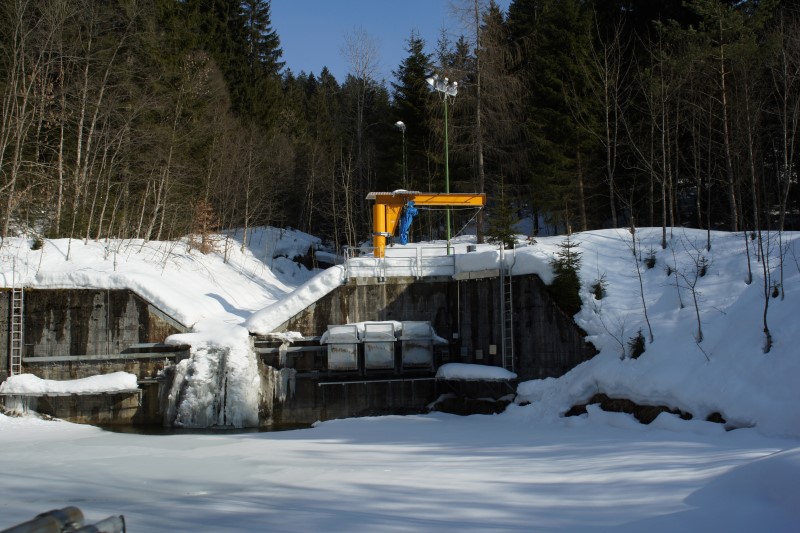
The research is based in the Erlenbach, a small river in the Alps that has been studied by Swiss researchers for several years. They have built a very sophisticated stream sampling station, which can capture everything that flows down past a gauging station. There is a large retention pond that catches the logs/pebbles/sediments and a shopping-trolley sized wire basket that can be moved into the middle of the stream to catch a particular time point (for example the middle of a large storm). The photo below was taken during winter when the river was frozen over, but you can see the v-shaped river channel, the three wire baskets ready to move into position to catch material, and the snow in the foreground covering the retention pond.
The sampling system in the Erlenbach River during winter
This sampling system led to Jens observing that there was a lot of CPOC coming down the river and piling up in the retention pond. A quick calculation suggested that this was a significant portion of the total carbon coming out of the river catchment, but the scientific consensus was that actually more carbon came through as fine particles than CPOC. An experiment was designed to test this.
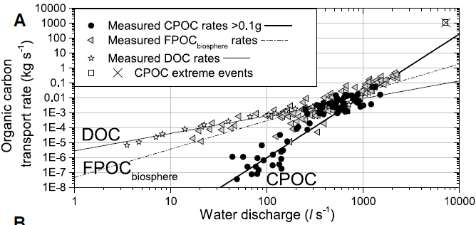
Across a wide range of river flow speeds, the amount and size of woody debris flowing down the river was measured, both waterlogged and dry material. This allowed a rating curve to be defined – that is for a given river flow speed, how much organic carbon would be expected to flow down the river? The rating curve was very biased towards the high-flow end for CPOC, much more so than for fine carbon (FPOC) or dissolved carbon (DOC). At low flow rates, very little CPOC is moved, but at high flow rates a very large amount is mobilised.
Rating curve of organic carbon types vs. river discharge
During the 31 years of data collection there were four particularly large storms. Integrating over the rating curve shows two things. Firstly, if the large storms are ignored then the Erlenbach is already a major source of CPOC, about 35% of the total carbon, with CPOC being roughly equal to the FPOC estimate. Thus it is much more important than might previously have been imagined. If the extreme events are included, the CPOC becomes ~80% of the total organic carbon transported by the river.
A majority of the CPOC transported by the river was waterlogged, having sat on the river bank or behind a log jam while waiting for a large storm to wash it downstream. Waterlogging increases the density of the wood and makes it more likely to sink when it reaches a lake or the sea. My contribution to the paper was to provide evidence of this process. My PhD work in the Italian Apennines found CPOC, from millimetre scale up to large tree trunks, that had been preserved in ocean sediments for millions of years. Again, a lot of this CPOC is too large to measure using standard techniques, and suggests that rivers can deliver organic carbon from mountains to the ocean far more efficiently than previously thought.
This paper is a result of collaboration with researchers at the University of Glasgow who I met while interviewing for a position. I didn’t get the job, but I did get talking to Paula Lindgren and we discovered a common interest in using Raman Spectroscopy to study organic carbon. This publication is the first result of that, and is available as an open-access article.
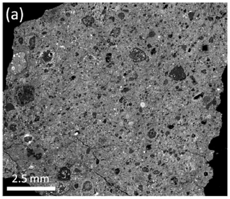
A little bit of meteorite, under an electron microscope
The paper is a comprehensive study of a meteorite collected from Antarctica. Antarctica is a great place to find meteorites because they sit on top of the ice and are easy to spot – sometimes the flow of ice even concentrates them into particular areas to makes things even easier. This meteorite is classified as a “CM carbonaceous chondrite” and has experienced very little change since it was part of the protoplanetary disc billions of years ago. Therefore we can use it like a time capsule to look at what the early solar system was like.
However, some meteorites are better time capsules than others. As they float around the solar system, they can build up ice, which can then be melted by radioactivity and the water released can alter the crystallography of the meteorite. Our paper uses a wide range of techniques to characterise the meteorite and show that it is one of the least altered carbonaceous chondrites ever found.
The techniques used included electron microscopy (both scanning and transmission techniques; SEM and TEM), X-ray analysis, X-ray diffraction, thermogravimetric analysis (TGA), oxygen isotope measurements and Raman Spectroscopy. My contribution was to use my automatic Raman processing technique to determine how crystallised the carbon in this meteorite was in comparison to carbon in other meteorites.
This paper, led by Josh West and colleagues in Taiwan, was published in Limnology and Oceanography. The full text is available via the journal website, since all L&O papers become open access after three years.
The island of Taiwan, in the South China Sea, has an interesting, yet devastating, combination of climate, biology and geology. It sits on the plate boundary between Eurasia and the Phillipines, which are moving into each other and causing the island to rise out of the ocean. This leads to earthquakes as the land is pushed up, and rapid erosion as the mountains get steeper and taller. The mountain sides collapse as landslides, producing sediment that is prone to being washed away by Taiwan’s many rivers. These rivers may not be the longest in the world, but they carry a lot of water, because Taiwan sits in the tropical zone where the year-round high levels of rainfall are topped up by several typhoons each year. The final piece of this jigsaw is the biology – being in a warm, wet region means that Taiwan is very biologically productive, with extremely fast forest growth rates.
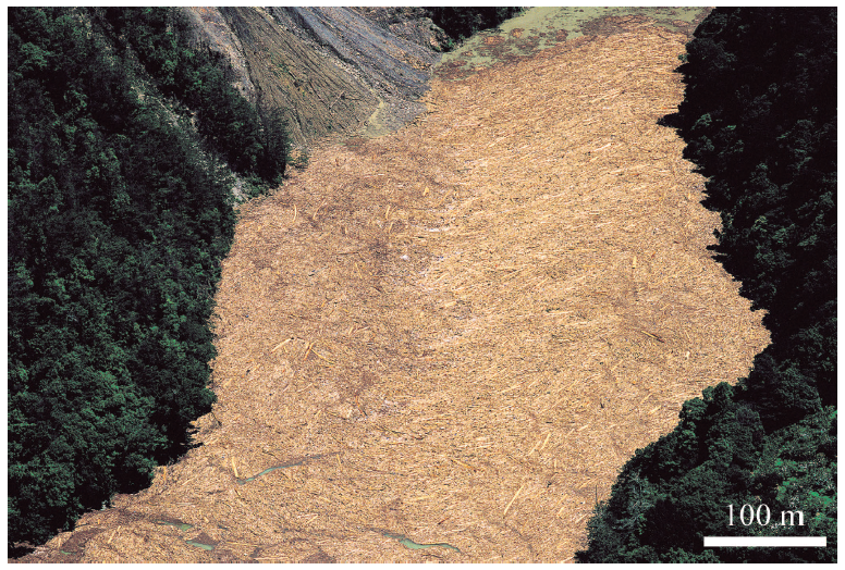
A Taiwanese reservoir after Typhoon Morakot
Coupling all of these features together leads to a heavily forested mountainous island on which the hillsides are regularly landsliding and generating woody debris (tree trunks, branches, shrubs etc.) The large typhoons that hit the island each year provide water which washes the woody debris into the rivers and then out to the ocean.
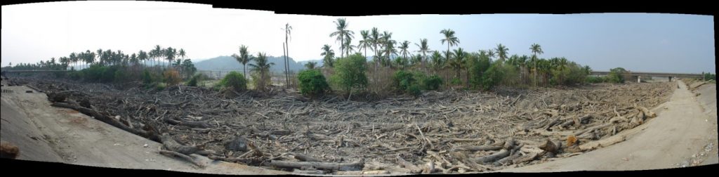
In 2009, Taiwan was struck by a particularly devastating tropical cyclone, Typhoon Morakot. The island received about 4 metres of rainfall in just a couple of days, enough to cause rivers to burst their banks, washing away entire villages and unfortunately leading to several deaths. I visited the island a few months later, and the clear-up operation was still going on. Beside the rivers was up to a metre of chaotic sediment with tree branches sticking out of it, since the waters had carried everything off the hillside and dumped it when the floods receded. A lot of the tree trunks made it all the way through the river, out to the sea. They washed up on the shoreline around Taiwan, and were reported as far away as Japan.
A Taiwanese river channel filled with logs after the storm
These trees contain a lot of carbon, which has been moved from the hillside to the floodplain and out to the sea. Our study tried to work out just how much carbon, in the form of coarse woody debris, was being transported during this storm. Single river channels, such as the picture above, could contain 40 million tonnes of carbon – how much carbon was washed away by the whole storm?
There were two independent methods used to make the carbon estimates. The first one compared aerial photography before and after the storm to look at how much area was affected by landslides, and how much of the island was covered in forest. If you combine the forest cover data with the landslide map, and correct for areas where landslides do not deliver the woody debris to the river network, an estimate of carbon mobilisation can be made
The second method used reservoirs as sampling facilities. Reservoirs have filters to stop large trees going through their exit pipelines, and so any woody debris reaching the reservoir will be stopped at the dam (see the top picture for an extreme example). Knowing the area of land that drains into the reservoir, and the amount of wood trapped at the dam, you can scale up to the area of the entire river catchment.
Both of these methods produced similar results, they agreed that there was a shocking amount of carbon washed to the ocean during the storm. The storm delivered 3.8 – 8.4 Teragrams of woody debris from Taiwan to the ocean, which represents 1.8 – 4.0 Teragrams of carbon. This is about 1/4 the annual delivery of carbon from the Amazon River, but most of that is as small particles. The woody debris delivery in these few days was over 10 times greater than the annual woody debris delivery from the Amazon. So one single event on a small island was significant from a global point of view, but how much carbon is a Teragram?
One Teragram is equal to one million tonnes; an oil tanker can carry 300 000 tonnes of oil (mostly carbon) and therefore the storm delivered 10 oil tankers worth of carbon to the ocean. Obviously this event is not as disastrous as an oil tanker spill – the woody material will rot down and provide food for ocean-living creatures as well as potentially being buried safely in the sediments.
Our paper shows just how much carbon can be washed away by a single storm, and highlights that large pieces of woody debris, too large to analyse by most techniques, are an important and probably under-studied element of the organic carbon cycle.
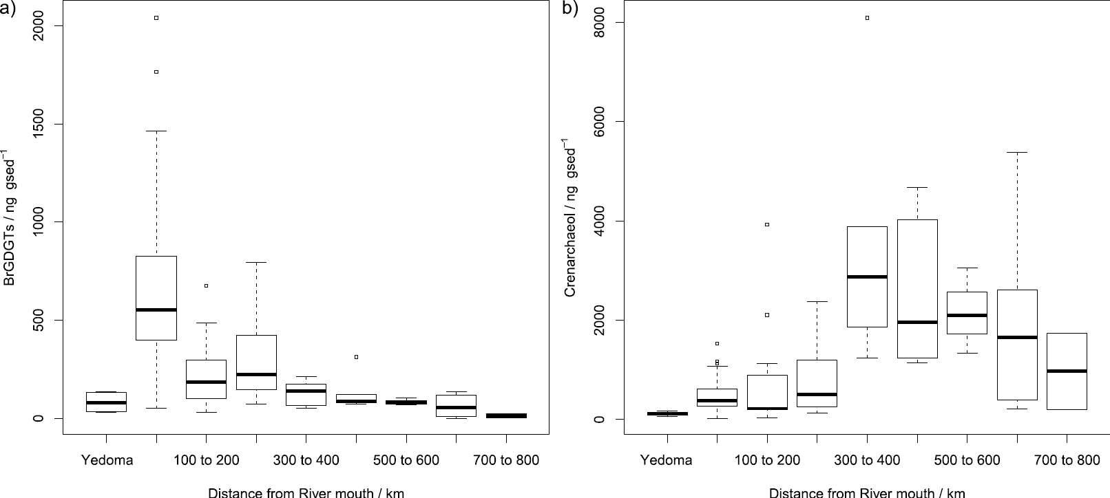
As I mentioned before, this paper has been submitted, reviewed and published completely open-access. This means that the original paper, the reviews and our response are all archived online forever. All of this is available freely to anyone, without the need to pay for access. You are free to copy, distribute and make use of the data and graphs as long as the original paper is cited (also known as a CC-BY copyright license)
Boxplots showing how GDGT biomarkers vary offshore
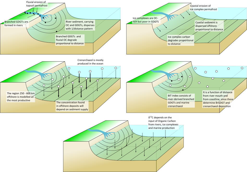
In the paper we show the first map of GDGT biomarkers from the East Siberian Arctic Shelf. This region is extremely remote yet very important within the global carbon cycle. Our work shows that this is an area of complex interaction between rivers, coastal erosion and open ocean productivity. The GDGT biomarkers are very useful here as a tracer of carbon being washed away by the rivers and being produced in the oceans, and this allowed me to make a model of the Arctic Ocean in this region to better understand how all of the different processes interact.
Our model of biomarker export across the Arctic Shelf
As an author, the publishing process for Biogeosciences was interestingly different. There was a reasonable amount of time between submitting the paper and final publication, but that was mostly due to the interactive public discussion stage which most journals do not have. During this time the paper was available and citable, which means that although it was relatively slow progress towards final publication the story was out there very quickly. I’m keen to go for this style of publishing again in the future.
I have recently had a paper accepted in the journal “Marine Geology“, which looks the transport of organic carbon during a major typhoon in Taiwan: “Redistribution of multi-phase particulate organic carbon in a marine shelf and canyon system during an exceptional river flood: Effects of Typhoon Morakot on the Gaoping River–Canyon system”.
Typhoon Morakot was a particularly severe tropical cyclone that hit the island in 2009, causing flooding, mudslides and hundreds of deaths. From an organic geochemistry perspective, it also transported sediment and organic carbon from the hillsides and floodplains out to the South China Sea. Some of this carbon was “fresh” material, coming from trees, grass, shrubs and soil. Other parts of the carbon was “fossil” carbon, sourced from the mountains running down the centre of the island, or from sedimentary rocks in the foothills and floodplains. It is important for the global carbon cycle to understand how much of the land-sourced (terrestrial) carbon makes it to the ocean floor, because this process can lead to carbon being stored in the sediments for millions of years.
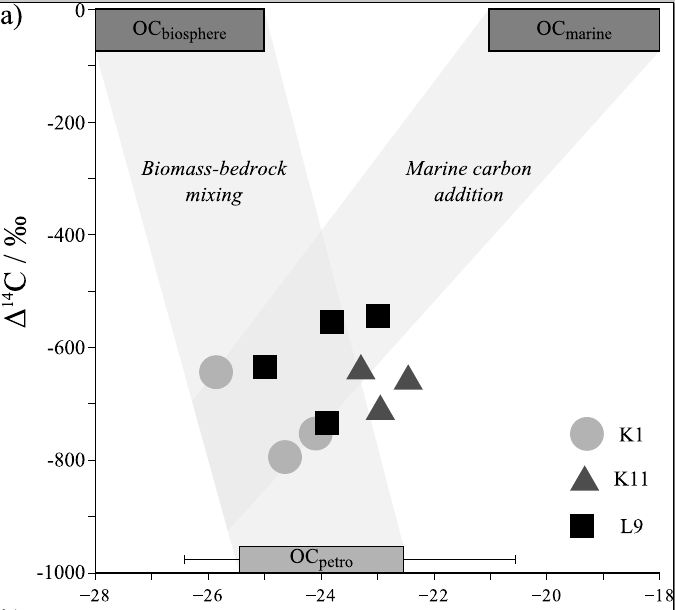
Out at sea, all of this organic carbon and sediment was mixed together with material produced in the water column, by algae and plankton. Mixing three carbon sources together makes it very difficult to work out how much of each one is present in a sample, which is where my work comes in. By combining measurements of the nitrogen to carbon ratio with the carbon-13 to carbon-12 isotope ratio, these three inputs can be identified. I did this for samples collected in the Gaoping Canyon, a deep submarine channel running from the island out to the deep sea. I found that terrestrial organic carbon was the dominant form of carbon present in the canyon and that therefore millions of tonnes of carbon were transported to and buried in the ocean by the typhoon.
Unmixing plant matter, bedrock OC and marine carbon
This carbon will most likely be locked away in these sediments for thousands or millions of years, while on the island more trees will grow to replace the ones washed away in the storm. In the process, carbon dioxide will be taken out of the atmosphere, so the storm-flood-burial cycle should go some way towards slowing the rate of climate change.
If you would like to download the paper, it is available freely via open access or as a PDF.
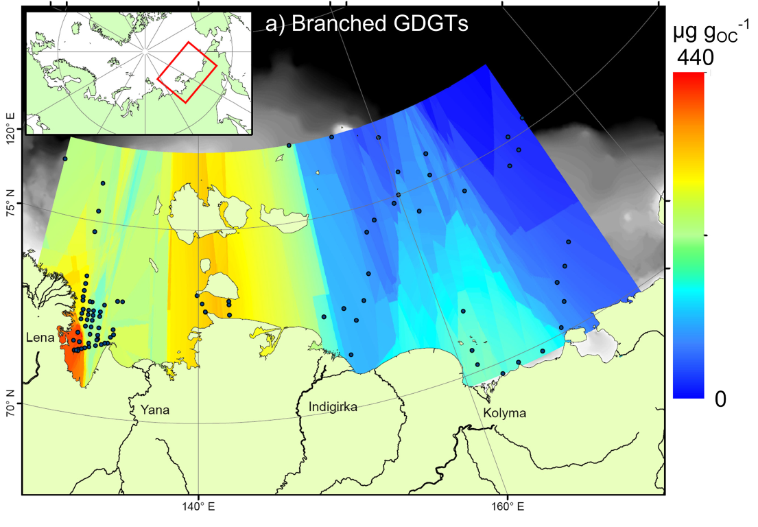
My last post talked about Open Access publishing, and the various philosophies for spreading (and/or making money from) academic knowledge. Now there is a chance to play an active part in the publishing process. My latest paper has been submitted to a journal called “Biogeosciences” which is administered by the European Geosciences Union (EGU). Their journals are published using a super open process, where more than just the final paper is released free-of-charge to the world. Whereas in regular Open Access publishing anyone is free to read the final reviewed work, in EGU journals the initial version is also made available. Two reviewers are selected from the community, and their reviews are shown on the website as well. Everyone else is free to read and comment on the paper, raising questions that the authors have to respond to. It is hoped that this system is a) transparent b) open to more (constructive) criticism than the standard two-review system and c) faster, since the paper is available for people to read at an earlier stage of the process.
A figure from the paper showing land-sourced GDGT molecules
Our paper discusses the distribution of GDGT biomarkers on the East Siberian Arctic Shelf. We measured these biomarkers to determine whether the organic matter deposited on the shelf came from land or ocean sources. When we had made these measurements, a model was created to try and explain the observations and work out the budget for carbon being delivered to the shelf from large Arctic rivers.
If you want to read and comment on the paper it is available on the Biogeosciences website
I will discuss Raman Spectroscopy in depth in a future post on this site, but the short version is that Raman allows me to determine the crystal structure of pieces of carbon within my samples. A river or marine sediment sample can be sourced from multiple areas, and mixed together during transport. Trying to work out where a sample was sourced from can prove very difficult. However, these source areas often contain carbon of different crystalline states; if I can identify the carbon particles within a sample then the sources of that sample, even if they have been mixed together, can be worked out. The challenge in this procedure is that there can be lots of carbon particles within a sample, and each one might be subtly different. To properly identify each mixed sample, lots of data is required, which can laborious to process.
Determining the types of carbon in a sample. Each spectrum is classified according to its peak shapes. Image (C) Applied Spectroscopy
My paper describes how lots of spectra can be collected efficiently from a powdered sediment sample. By flattening the powder between glass slides and scanning the sample methodically under the microscope, around ten high-quality spectra can be collected in an hour, meaning five to ten samples can be analysed in a day. Powdered samples are much easier to study than raw, unground, sediment, and I have shown that the grinding process does not interfere with the structure of the carbon particles, therefore it is a valid processing technique.
Once the data has been collected, I have devised a method for automatically processing the collected spectrum using a computer, which removes the time-consuming task of identifying and measuring each peak by hand. The peaks that carbon particles produce when analysed by Raman Spectroscopy have been calibrated by other workers to the maximum temperature that the rock experienced, and this allows me to classify each carbon particle into different groupings. These can then be used to compare various samples, characterise the source material and then spot it in the mixed samples.
Delegating as much analysis as possible to a computer ensures that each sample is treated the same, with no bias on the part of the operator, and also cuts down the time required to process each sample, which means that more material can be studied. The computer script used to analyse the samples is freely available and therefore other researchers can apply this to their data, enabling a direct comparison with any samples that I have worked on. This technique will hopefully prove useful to more than just my work in the future, and anyone interested in using it is welcome to contact me. While the paper discusses my application of the technique to Taiwanese sediments, I have already been using it to study Arctic Ocean material as well.
The paper itself is available from the journal via a subscription, and is also deposited along with the computer script in the University of Manchester’s open access library.
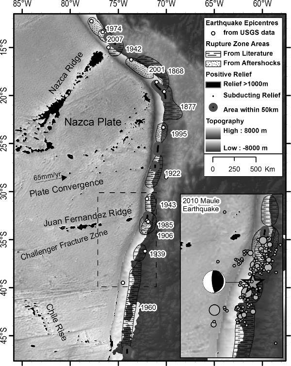
The initial observation for this work was that ‘great’ earthquakes, those which measured more than magnitude 8.0, tend to have end points in the same place. An earthquake end point is the limit to the earthquake fault plane movement, shaking will take place outside of this zone but it is most violent in the regions above the fault plate movement. The figure below shows the rupture zones and end points for great South American earthquakes.
Rupture zones and subducting topography in South America
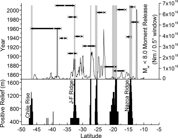
An initial inspection of the plate margin (where the incoming Pacific Plate is subducted underneath the South American Plate) suggested that when there are underwater mountains on the Pacific Plate coming into the subduction zone (black blobs on the figure above), these tend to match up with the end points of earthquakes. The figure below shows how topographic features (underwater mountains and ridges) match up with earthquake locations.
Subducting topography and earthquake locations
To test whether this was a real relationship, or just coincidence, I designed a model that produced earthquakes along the subduction zone. The model had two versions. In version one, earthquakes were placed in line along the subduction zone (as tends to happen in these situations, one earthquake starts at the end point of a previous one) but their end points were not constrained by anything. In the second version, if the earthquake tried to rupture past an incoming topographic feature, the rupture was stopped there.
By applying statistical tests to the model, I showed that the endpoints of earthquakes were far more likely than random chance to be located where topography > 1000m was being subducted. The model also showed that subducting topography led to a reduction in background earthquakes. At earthquake endpoints not associated with topography, there was an increased amount of smaller earthquakes releasing the built-up stress, but this was not seen at earthquake endpoints near to subducting topography. Therefore, subduction of a high seamount or ridge makes the subduction zone earthquake activity decrease (it becomes ‘aseismic’) which prevents both great earthquakes getting past, and smaller earthquakes from occurring.